PHY 310: Computational Physics Projects

What I Did

• ODE solvers (harmonic/anharmonic, driven/chaotic)
  Implemented explicit Euler, semi-implicit (symplectic) Euler, RK2/Heun, and RK4. Verified convergence by fitting the error model for RK4. Checked energy drift on Hamiltonian systems, showing symplectic Euler better preserves (H(q,p)) over long horizons.

• Chaos & bifurcations
  Generated the logistic-map bifurcation diagram and estimated the Lyapunov exponent. Integrated the Lorenz system:

  $$\dot{x}=\sigma(y-x),\quad \dot{y}=x(\rho-z)-y,\quad \dot{z}=xy-\beta z$$

  and visualized the strange attractor + return maps.

• Finite differences (PDE/eigenproblems)
  Discretized the 1D time-independent Schrödinger equation

  $$-\frac{\hbar^2}{2m}\frac{d^2\psi}{dx^2}+V(x)\psi=E\psi$$

  with 2nd-order central differences, forming a tri-diagonal system solved efficiently. For an infinite well of width, verified equation and node counts of eigenfunctions.

• Spectral/FFT tools
  Used FFTs to analyze frequency content, compare spectral vs. FD resolution at equal grid sizes, and sanity-check Parseval-style energy consistency in time series.

• Monte Carlo
  Implemented MC integration with importance sampling; confirmed error scaling on log–log plots and observed variance reductions on suitable test integrands.

• Performance & correctness
  Vectorized inner loops with NumPy; profiled hotspots. Added lightweight checks (convergence orders, conservation laws) to prevent regressions.

• Visualization & reporting
  Reusable Matplotlib helpers (phase portraits, bifurcations, error curves). Each notebook ends with Takeaways summarizing stable parameter ranges and method trade-offs.

Methods & Experiments (Examples)

• Pendulum / Mass–Spring (ODE)
  Small-angle model: $\ddot{x} + \omega^2 x = 0$.
  Nonlinear pendulum:

  $$\ddot{\theta}+\frac{g}{\ell}\sin\theta=0,\qquad E=\tfrac12 m\ell^2\dot{\theta}^2 + m g \ell\,(1-\cos\theta).$$

  Step-size sweep $h \in [10^{-4},\,10^{-1}]$: measured $L^2$ error vs. analytic solution; compared long-time energy behavior (RK4 baseline vs. symplectic Euler).

• Lorenz Attractor (Chaos)
  Parameters $\sigma=10,\ \rho=28,\ \beta=8/3$. RK4 with adaptive-step trials; separation of nearby trajectories to visualize sensitivity; Poincaré/return maps.

• Schrödinger (FD eigenproblem)
  Infinite well and finite barrier; verified second-order convergence by halving $\Delta x$ and observing $\approx 4\times$ error reduction.

• Monte Carlo Integration
  Estimated $\pi$ and multi-D integrals; compared plain vs. importance sampling; confirmed $\lVert \hat{I}-I \rVert \propto N^{-1/2}$.

Results (Quick Snapshots)

• RK4 achieved $\sim\!\mathcal{O}(h^{4})$; symplectic Euler showed qualitatively superior long-time energy behavior.
• FD eigenvalues matched analytics to $<\!1\%$ at moderate grids; errors halved when $\Delta x$ halved (2nd order).
• MC variance improved $2\!-\!3\times$ under importance sampling on selected integrands.

Additional Images (Gallery)

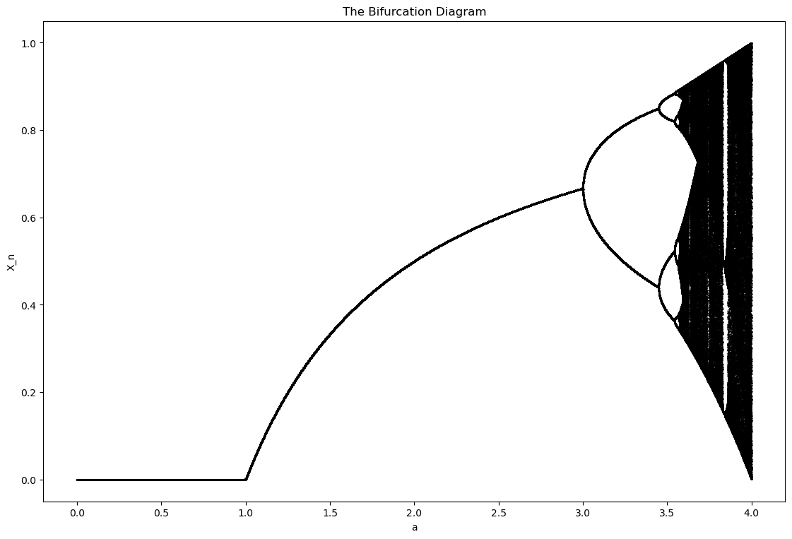Logistic-map bifurcation diagram (period-doubling route to chaos).

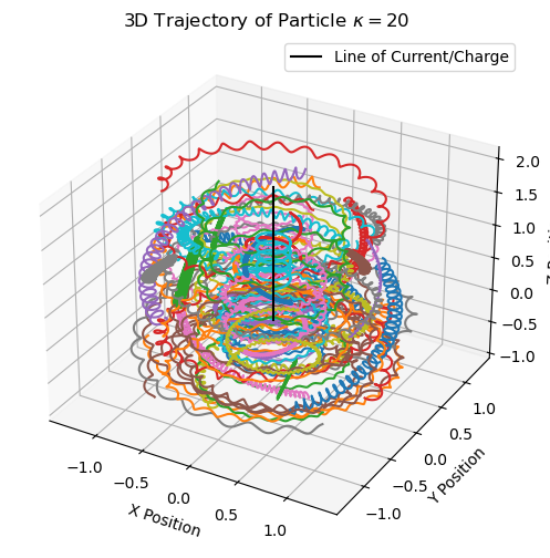Lorenz attractor integrated with RK4; color encodes $\kappa$ state particle around a electromagnetised charged line.

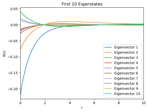First few eigenstates for a 1D infinite square well (FD discretization).